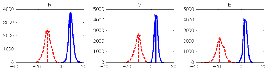
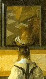
Top (Target Color Space)

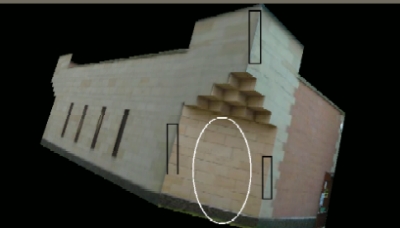
Left (Before)
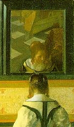
Right (Before)
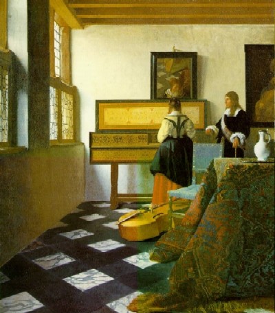
Whole (Before)
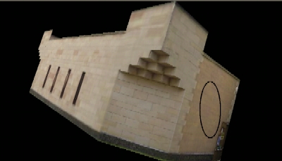
Top (Target Color Space)
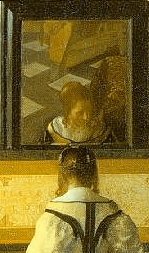
Left (After)
Right (After)
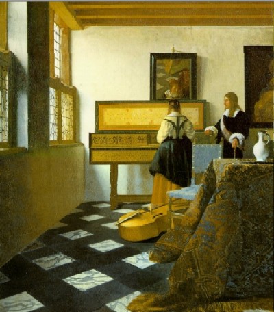
Whole (After)
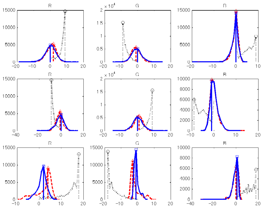
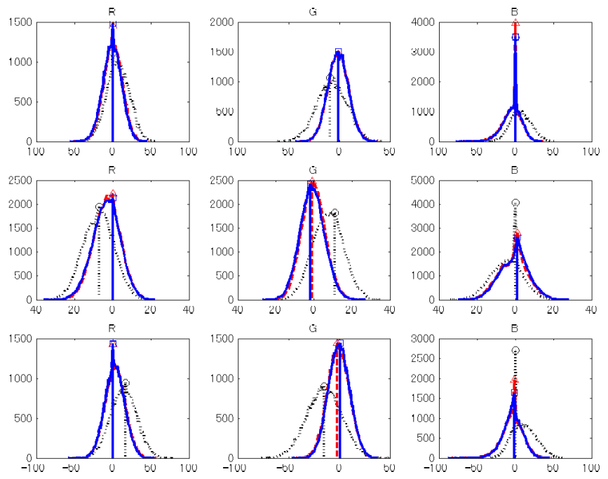
| Before the Multiple Color Image
Fusion |
After the Multiple Color Image
Fusion |
|
Top (Target Color Space) Left (Before) Right (Before) Whole (Before) |
Top (Target Color Space) Left (After) Right (After) Whole (After) |
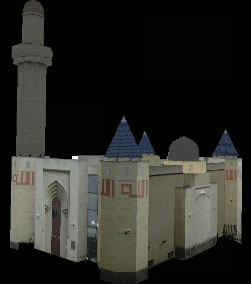
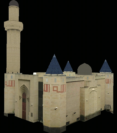
| Before the Multiple Color Image
Fusion |
After the Multiple Color Image
Fusion |
|
Top (Target Color Space) 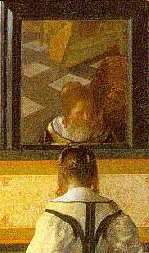 Left (Before)  Right (Before) 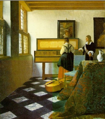 Whole (Before) |
Top (Target Color Space)  Left (After) 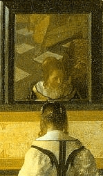 Right (After) 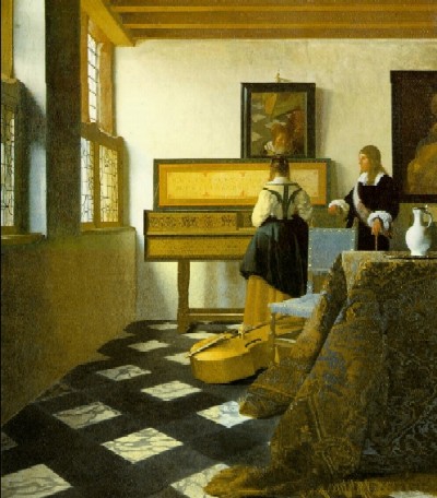 Whole (After) |
| Before the Multiple Color Image Fusion | After the Multiple Color Image Fusion |
 |
 |
| Before the Multiple Color Image Fusion | After the Multiple Color Image Fusion |
 |
 |
| Before the Color Image Fusions | After the Multiple Color Image Fusion | After the Pairwise Color Image Fusion |
 Image 1 (Target Color Space)  Image 2 (Before)  Image 3 (Before)  Image 4 (Before)  Image 5 (Before)  Image 6 (Before)  Image 7 (Before)  Image 8 (Before) |
 Image 1 (Target Color Space)  Image 2 (After Multiple)  Image 3 (After Multiple)  Image 4 (After Multiple) 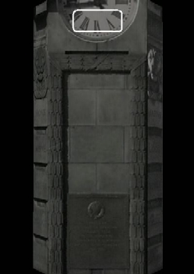 Image 5 (After Multiple) 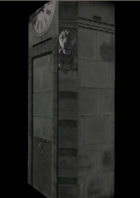 Image 6 (After Multiple)  Image 7 (After Multiple) 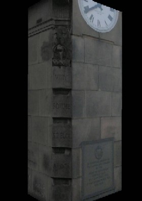 Image 8 (After Multiple) |
 Image 1 (Target Color Space)  Image 2 (After Pairwise)  Image 3 (After Pairwise)  Image 4 (After Pairwise)  Image 5 (After Pairwise) 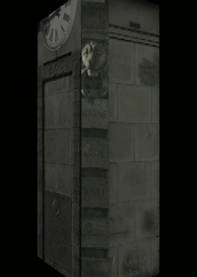 Image 6 (After Pairwise) 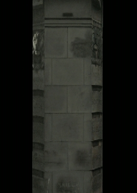 Image 7 (After Pairwise) 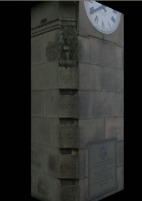 Image 8 (After Pairwise) |